
Michigan Technological University Michigan Technological University
Digital Commons @ Michigan Tech Digital Commons @ Michigan Tech
Dissertations, Master's Theses and Master's
Reports - Open
Dissertations, Master's Theses and Master's
Reports
2014
FAULT MORPHOLOGY WITHIN THE SOUTHERN KENYAN FAULT MORPHOLOGY WITHIN THE SOUTHERN KENYAN
PORTION OF THE EAST AFRICAN RIFT VALLEY PORTION OF THE EAST AFRICAN RIFT VALLEY
Justin B. Wargelin
Michigan Technological University
Follow this and additional works at: https://digitalcommons.mtu.edu/etds
Part of the Geology Commons
Copyright 2014 Justin B. Wargelin
Recommended Citation Recommended Citation
Wargelin, Justin B., "FAULT MORPHOLOGY WITHIN THE SOUTHERN KENYAN PORTION OF THE EAST
AFRICAN RIFT VALLEY", Master's report, Michigan Technological University, 2014.
https://doi.org/10.37099/mtu.dc.etds/821
Follow this and additional works at: https://digitalcommons.mtu.edu/etds
Part of the Geology Commons
FAULT MORPHOLOGY WITHIN
THE SOUTHERN KENYAN PORTION OF THE EAST AFRICAN RIFT
VALLEY
By
Justin B. Wargelin
A REPORT
Submitted in partial fulfillment of the requirements for the degree
of
MASTER OF SCIENCE
In Geology
MICHIGAN TECHNOLOGICAL UNIVERSITY
2014
(c) 2014 Justin B. Wargelin

2
This report has been approved in partial fulfillment of the requirements
for the Degree of MASTER OF SCIENCE in Geology.
Department of Geological/Mining Engineering and Sciences
Report Advisor: James R. Wood
Committee Member: Carol A. MacLennan
Committee Member: Alexandria L. Guth
Department Chair: John Gierke
3
Dedication:
To Professor William Gregg who was my Co-Advisor before his death and who
motivated me as to questions about geology; and to Professor Jim Wood for
introducing me to the East Africa Rift and for persevering with me through the
completion of the report.
4
Table of Contents
Introduction: Goals and Hypotheses . . . . . . . . . . . . . . . . . . . 8
Geologic Setting and Background . . . . . . . . . . . . . . . . . . . . . 13
Method Development . . . . . . . . . . . . . . . . . . . . . . . . . . . . . . . 16
Results and Discussion: Data and Observations . . . . . . . . . 21
Limitation of Research and Future Work . . . . . . . . . . . . . . . . . 34
Conclusions . . . . . . . . . . . . . . . . . . . . . . . . . . . . . . . . . . . . . . . 36
Bibliography . . . . . . . . . . . . . . . . . . . . .. . . . . . . . . . . . . . . . 38
Appendices . . . . . . . . . . . . . . . . . . . . . . . . . . . . . . . . . . . . . . . 40
5
List of Figures
Figure 1: Southern Kenyan Rift 8
Figure 2: Map Showing Outline of Africa and the Middle East 9
Figure 3: Map Showing the Traces of Faults Mapped for This Study 10
Figure 4a: Southern Kenyan Rift Valley 12
Figure 4b: Southern Rift Valley near Nairobi 13
Figure 5: Method 1: Example of Breaking Fault Scarps Profiles into 18
Segments - Fault 1a Profile
Figure 6: Method 1: Fault 1a Segment 1 Profile with Excel Linear 19
Trendline
Figure 7: Theoretical Model of Scarp Erosion--Fault 1a Profile 22
Figure 8: Fault 3J: Corrected for VE 24
Figure 9: Fault 5i as Drawn by Excel: Original VE 25
Figure 10: Fault 5i as Drawn by Excel: Corrected for VE 26
Figure 11: Fault 2n as Drawn by Excel: Original VE 27
Figure 12: Fault 2n as Drawn by Excel: Corrected for VE 27
Figure 13: Buckley et al. Explanation of Development of Loriu 28
Escarpment
Figure 14: Fault 6a as Drawn by Excel: Original VE 30
Figure 15: Fault 6a as Drawn by Excel: Corrected for VE 30
Figure 16: Fault 6a Possible Interpretation 31
Figure 17: Fault 6e as Drawn by Excel: Original VE 32
Figure 18: Fault 6e as Drawn by Excel: Corrected for VE 33
Figure 19: Fault 6e Possible Interpretation 34
Figure 20: Theoretical Model of Scarp Erosion--Fault 1a Profile: 40
VE Example
Figure 21: Fault 1a corrected for VE 41
6
Acknowledgements
This research project came about because of my brief visit to the area in May of 2008
when I participated in an East African Field Geology course/trip with Dr. James Wood
of the Michigan Technological University Geology Department. For the first two
weeks of the trip, we stayed in Nairobi, exploring the Rift Valley and the area around
Lake Magadi. During the third week we went on "safari" traveling up the Rift Valley to
see several of the lakes above Lake Magadi and staying along the lakes themselves.
This included Lakes Naivasha, Baringo, Bogoria and Elementaita in that order,
seeing Elementaita on the way back to Nairobi. We explored the escarpments and
visible fault scarps around this Lake Magadi region. I became interested in how these
fault scarps could be studied from afar-as well as on the ground.
I also wish to credit Alexandria Guth for providing me with a valuable tip for tracing
faults in the same direction with respect to dip direction, as my shapefiles in Global
Mapping were created.
7
Abstract
Faults form quickly, geologically speaking, with sharp, crisp step-like profiles. Logic
dictates that erosion wears away this "sharpness" or angularity creating more
rounded features. As erosion occurs, debris accumulates at the base of the scarp
slope. The stable end point of this process is when the scarp slope approaches an
ideal sigmoid shape.
This theory of fault end process, in combination with a new method developed in this
report for fault profile delineation, has the potential to enable observation and
categorization of fault profiles over large, diverse swaths of fault formation-- in remote
areas such as the Southern Kenyan Rift Valley. This up-to date method uses remote
sensing data and the digitizer tool in Global Mapper to create shape files of fault
segments.
This method can provide further evidence to support the notion that sigmoidal-
shaped profiles represent a natural endpoint of the erosional process of fault scarps.
Over time, faults of many different ages would exist in this similar shape over a wide
region. However, keeping in mind that other processes can be at work on scarps--
most notably drainage patterns, when anomalies in profiles are observed,
reactivation in some form possibly has occurred.
8
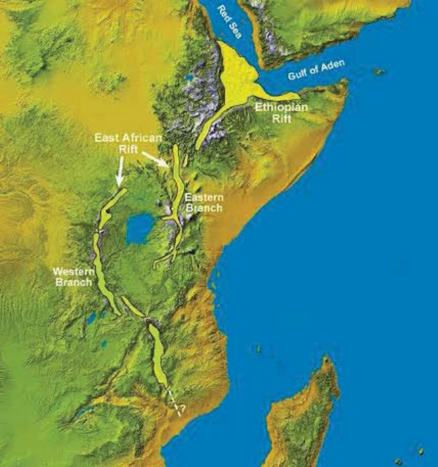
Introduction: Goals and Hypotheses
The purpose of this study is to develop a method for examining the geomorphology
of the fault-bounded horst blocks in the Southern Kenyan Rift (Fig. 1). In this and
other more remote and inaccessible areas, applied remote sensing techniques can
prove invaluable when, as often is the case, the resources are lacking to fund more
traditional methods of surveying large areas.
Figure 1: Southern Kenyan Rift
Source: Courtesy of Alexandria Guth

9
Figure 2: Map Showing Outline of Africa and the Middle East
Box indicates area of study shown in map on following page.
10
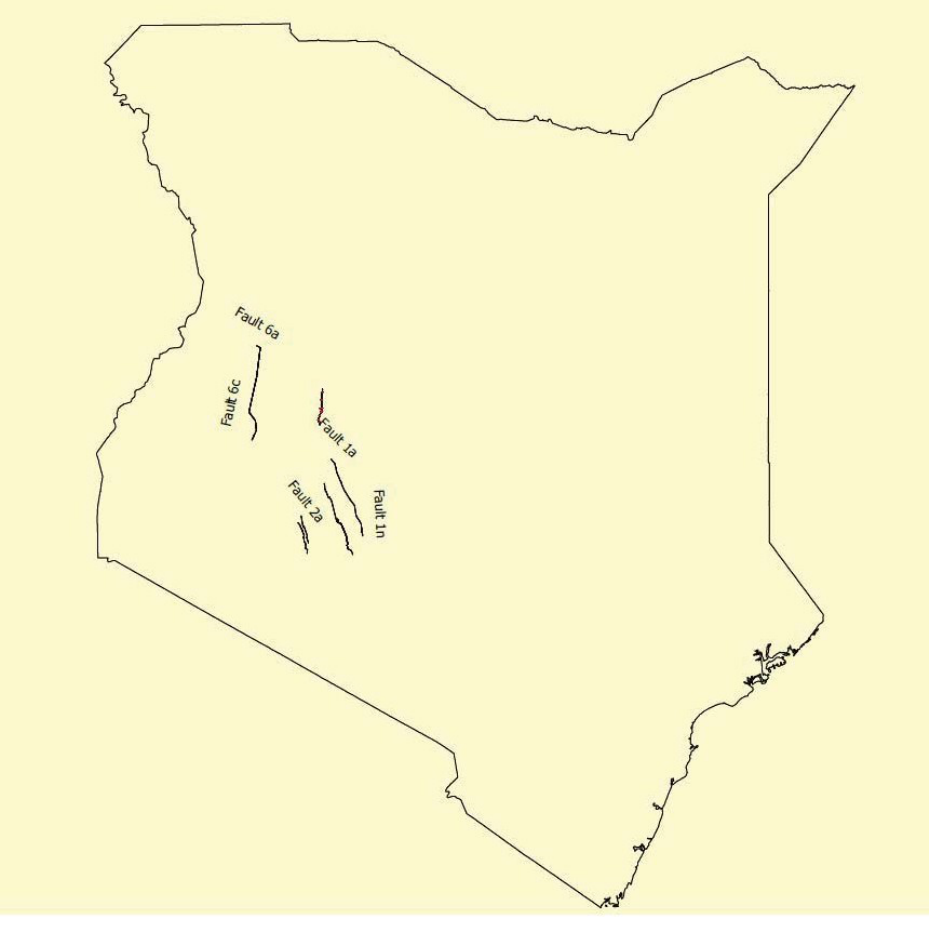
Figure 3: Map Showing the Traces of Faults Mapped for This Study
Western border of Kenya on left
11
A secondary long term purpose of this report is to use the methods developed to
examine the morphology of fault scarps within the Rift Valley for similarities in how
they are aging/eroding in hopes of gaining insights into the geologic history of the rift.
This is an aspect of the Southern Kenyan rift valley that has not received much
attention with the exception of recent work by Gloaguen et al. 2007 and Sequar,
2009, both of whom used remote sensing for classifying general geological structure.
A detailed understanding of how these features erode and change over time could
provide new insights into the rift's geologic history, perhaps even leading to a better
understanding of the sequence of the faulting events that define the southern rift. If
the scarps were found to trend towards a given end state of erosion, then their
relative "distance" from this state could speak to their relative age (i.e. a "pristine"
fault that is close to its original post-movement state could be assumed to be younger
and perhaps have seen more recent activity than one that was further along towards
the theoretical erosion end-state.) This would provide insight into the sequence of
faulting if faults with some orientations appeared older than others of a different
orientation; the older orientation could represent an early stress state of the regional
crust. It's also possible that the scarps could provide some indication of reactivation
in later phases of the overall rifting sequence. In such a case, an initial period of
movement on the fault would be followed by erosion during a period of quiescence
before later reactivation of the fault. This quiescent period would have an impact on
the geomorphology of the scarp. Most likely this would show itself in the scarp and
show different ages across its profile. The larger overall profile of the scarp may
reflect the original faulting and queasiest period of erosion, while the portion of the
scarp nearest the fault itself would reflect the later reactivation and subsequent
erosion.
Since the faults in this region have been measured as being relatively steep, -70°-
80°, and thus significantly steeper than the angle of repose, it's likely that scarps
would have two different slopes reflecting the different ages of the faulting events that
12
created the slopes to begin with. These are the main concepts involved in this
investigation.
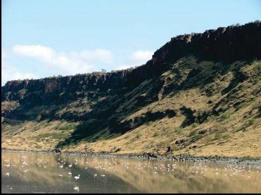
As noted, the estimated slope angles of most of the faults in the study area have dips
of -70°-80°. The general appearance of the landforms, including the horst blocks is
illustrated in photographs in Figures 4a and 4b.
Figure 4a: Southern Kenyan Rift Valley
[Both pictures 4a and 4b are of the Southern Kenyan Rift Valley courtesy of Alexandria Guth]
13
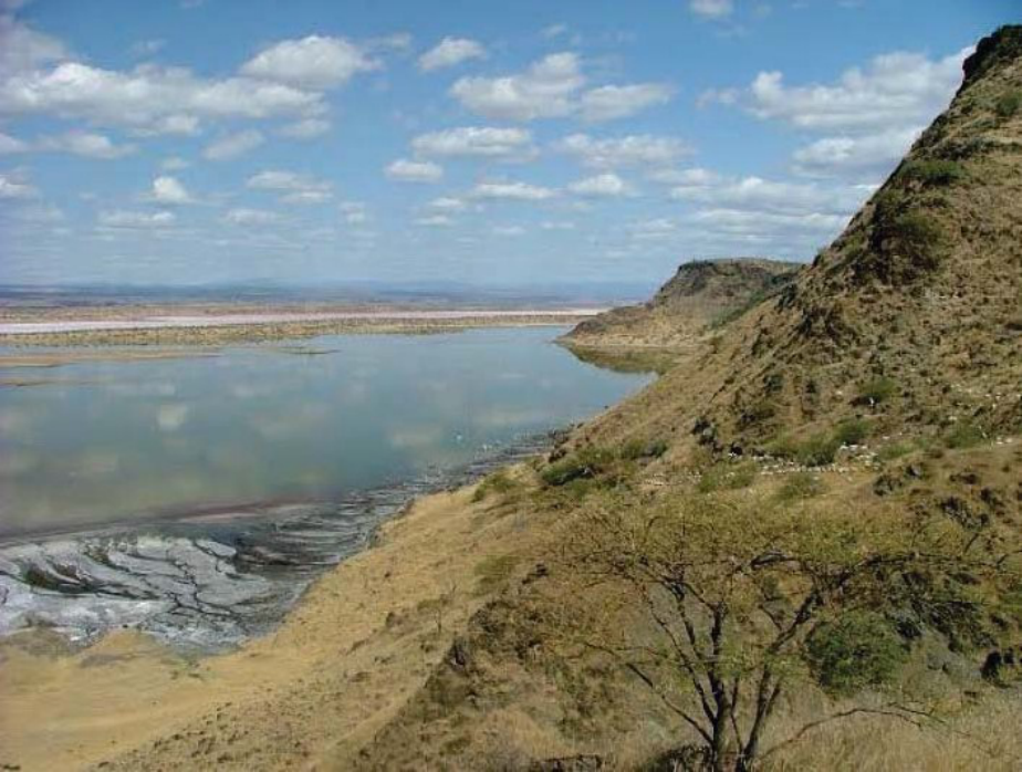
Figure 4b: Southern Rift Valley near Nairobi
The geological and research background of the horsts blocks in this region will be
described in the following section, followed by a description and discussion of how a
remote sensing method was developed for studying fault profiles, prior to presenting
data observation, interpretations, and findings.
Geologic Setting and Background
Rifts (areas where the Earth's crust is spreading or lengthening, and thus thinning)
are one of the most spectacular features of global morphology. Within oceans they
are locations where separate plates move apart (driven by convection within the
Athenosphere) as new oceanic crust is created. Of all the world's rifts none can
match in scale and diversity the Great Rift System, which runs for over 7000 km and
includes the East African Rift System and its extension through the Red Sea into the
14
Dead Sea, to form a unique feature of global geology. This forms (with the exception
of Iceland) the only place on Earth where a Divergent Plate boundary can be
accessed on land; where it is far easier to field work and conduct scientific
investigation. The East African Rift system represent a fairly early stage in the
evolution of such plate boundaries, including the thermal, magmatic, and tectonic
processes which gave rise to them (H.G. Reading, 1986, p.1). Thus, It is one of the
best examples of an active rift that exists today and has been used to interpret older,
subsurface basins worldwide. (Frostick, 1997, p.187)
The Southern Kenyan rift represents a major part of the East African rift system.
Baker (1987) identified three major stages in the tectonic development of the Kenyan
rift:
(1) The pre-rift stage (30-12 Mya) with the forming of a depression and minor
faulting
(2) The half-graben stage (12-4 Mya) with the forming of the main boundary
faults, and
(3) The graben stage (4 Mya - Present) with an increase and an inward
migration of faulting.
All stages were accompanied by intense, mostly alkaline, volcanism. However,
almost all volcanoes of the Southern Kenyan rift are now extinct with some post
volcanic hydrothermal activity in many places (M. Ibs-von Seht et al. 2008, p.69).
The Southern Kenyan rift valley consists of numerous fault blocks encompassing
horsts, grabens and step-fault platforms that are very little modified by erosion
(Baker, 1953, p.1). Fischer, Thomson, and Von Honhel in 1883 were the first
Europeans to publish regarding expeditions to the Magadi area. They passed along
the foot of the Nguruman escarpment in April, 1883 and noted the abrupt cliffs and
banded terraces. In 1913, Parkinson described the fault escarpments and horsts or
fault blocks in the Magadi region. (Baker, 1958, p.3) The soils on the lava horsts
were described as generally thin and patchy. Since this era, the intensity of research
in the area has waxed and waned over the succeeding decades, reaching a peak
during the 1970s and early 1980s when many of the most important hominid sites
15
were found (Leakey et al. 1976).
The Kenyan rift valley raises formidable questions about the regions geologic history.
Notably the Late Miocene and Late Pliocene to Mid-Pleistocene phases of
dominantly phonolitic and trachytic activity coincided with periods of strong uplift of
the Kenyan swell and with periods of rift-faulting. On the other hand, the Miocene
and Pliocene basaltic volcanism occurred at times of comparative crustal stability.
These features indicate a degree of interdependence of tectonic activity and
volcanism that support the view that both processes are expression of surface
changes in the upper mantle. (Baker, 1971, p.213).
As with all geological linear or curvilinear features, rifts are not the continuous simple
features they appear to be when looked at from afar. They are invariably broken into
segments by transverse features. The larger the scale at which they are seen, the
more complex they become. Individual segments vary considerably in their structural
style. Not only are rifts asymmetric in cross-section, but the direction of asymmetry
appears to vary systematically along the rift, with the direction of asymmetry
alternating between Eastern and Western Escarpments (Baker, 1988, p. 4). For a
given age, length of faults, width of rift basins, relief of the uplifted rift flanks vary
depending not on the age but on the stage of the rift segment (Chorowicz et al. 1987,
p. 400).
One of the first remote sensing evaluations of fault blocks was conducted by
Gloaguen et al. in 2006. This investigation showed that using radar, data on faults
can be sufficiently detailed for the purpose of geologic mapping. This allowed an
unbiased and fast counting of faults for further statistical analysis. However, faults
were evaluated as sets of connected segments. The goal was to use this data to
propose an evolution model for the growth, interaction and linkage of faults. (R.
Gloaguen et al. 2007, p. 137)

16
In 2009, Sequar used remotely sensed datasets along with other subsurface and
surface data to characterize faults in the Lake Magadi area. Combined results of
these datasets revealed four fault sets in the area. The existence of four set of faults
having different styles and different relative ages suggested dynamic changes in
tectonics of the Southern Keynan rift over time. (Sequar, 2009, p.1)
Thus, the value of remote sensing data for further exploring the geomorphology of
the fault-bounded horst blocks in the Southern Kenyan Rift valley has been firmly
established. This report develops and documents a new and up-to-date method for
mapping fault segments, using remote sensing data and the digitizer tool in Global
Mapper to create shapefiles of fault segments.
Method Development
The method devised uses MRSID LANDSAT images (available online at NASA's
"Geocover" Website https://zulu.ssc.nasa.gov/mrsid) and SRTM (Shuttle Radar
Topography Mission) elevation data available through Global Mapper's data
download system. Combining this data together within Global Mapper 9 and 10 (the
latter was released in 2010 while the research was underway) faults were digitized,
breaking them up into straight-line segments using the digitizer tool. That is to say
that any lineations with a significant slope were mapped as a single feature that
zigged and zagged back and forth for as long as it continued.
Original Method
The original method used the topographic profile tool within Global Mapper to
generate elevation profiles running perpendicular to the fault segments, saving the
profiles as distance versus elevation text files (.xz). These files were then imported
into Excel and saved after pasting in the "path details" from both the profile and a
smaller profile that was used to take the fault scarp slope at the steepest point in full
profile. Global Mapper's "path details" includes the "tilt" measurement which gives
17
the slope of any profile made in the program. However, this measurement is taken
from one end point to the other, making a second smaller profile necessary to
measure from the steepest point. With this method, the slope has to be found by
plotting the steepest part of the scarp (the part inferred to be a remnant scrap) in
Excel and using Excel's trendline feature to get an equation for the trendline of the
form:
Y=mX+A
Where: Y=elevation, m= slope, x=distance, and A= the starting elevation of the slope
Once this slope trend was determined, the inverse tangent can be computed to get
the slope's angle in degrees, since m is really just the tangent of the slope.
Unfortunately, this original method required that the slope be measured at several
different points along the scarp profile.
An example of how this worked from a fairly typical fault in the Magadi area of
southern Kenya follows on the next page.
18
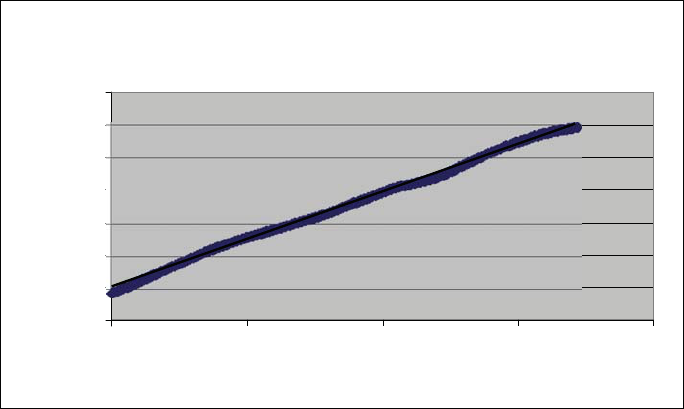
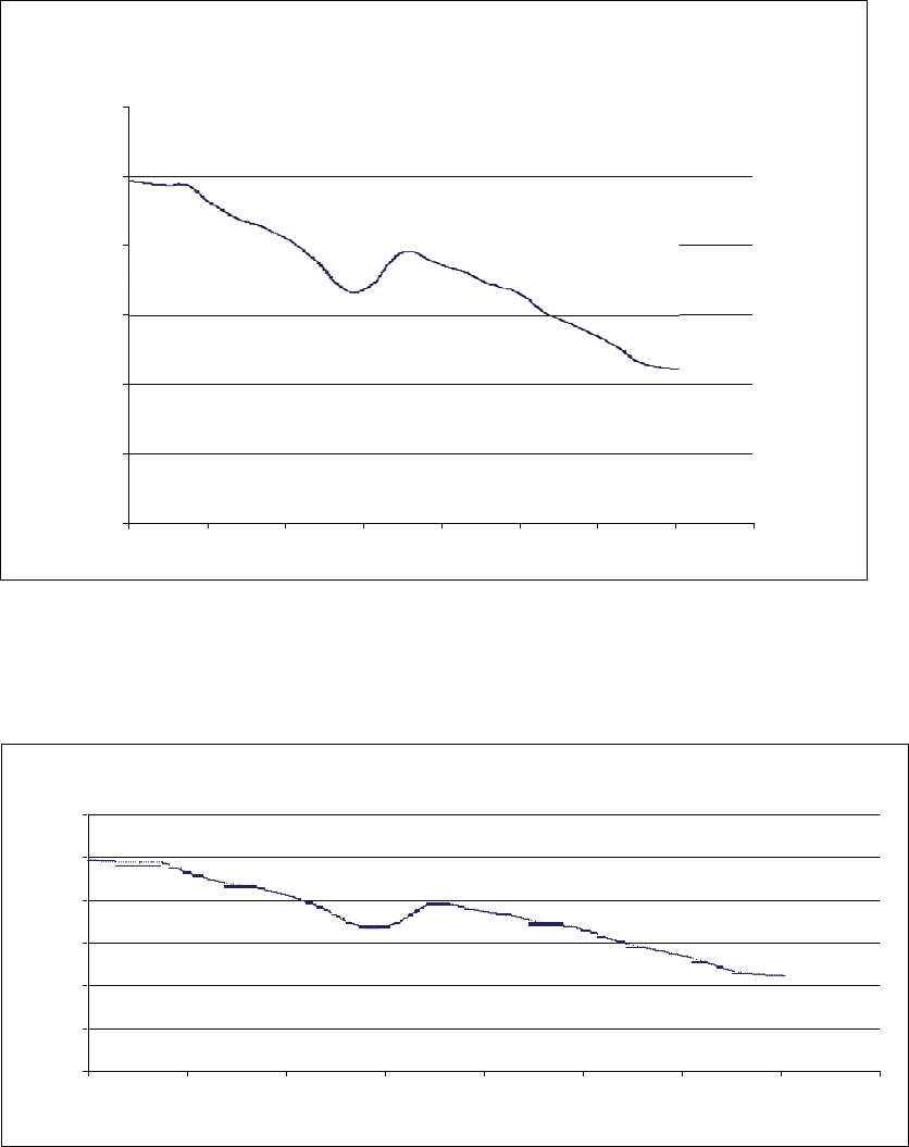
Figure 5: Method 1: Example of Breaking Fault Scarps Profiles into Segments
Fault 1a Overall Method 1 Profile
All units are in meters throughout this paper
.
Starting with the distance/elevation files, these were exported into Global Mapper as
".xz" text files and then imported into Excel to generate the graph above. For this
example, the slope on the uphill side of the fault (in this case. east of the fault) was
detailed. This is slope segment 1. Slope segment 2 is the steepest part of the scarp
itself and slope segment 3 is the debris pile that has built up at the bottom of the
scarp.
Fault1a Profile
2460
2440
2420
2400
2380
2360
2340
2320
0500 1000 1500 2000 2500
Distance
(
m
)
Elevation
(m)
19
Figure 6: Method 1: Fault 1a Segment 1 Profile with Excel Linear Trendline
A linear trendline was then developed with its equation displayed. This was then
converted into the trend line's slope in degrees using the following equation:
Excel formats its linear trendlines as:
Y=slope *X + Constant
The constant sets the line's vertical position on the graph:
Slope = Rise/Run = tane (slope in degrees) therefore 8=Atan (slope)
For the Method 1 example above, Excel gives a trendline with a slope of 0.0736, so
the calculations for slope segment 1 are as follows:
slope = 0.0736
Tan8= rise/run =slope=0.0736
tan8=0.0736
8=Atan(0.0736)=4.20938°
Fault 1a Se
g
ment 1
2450
2440
2430
2420
2410
2400
2390
2380
y
= 0.0736x+ 2390.2
0 200
400
Distance(m)
600 800
Elevation(m)

20
Given that segment 1 was defined as being the top of the footwall block, a low slope
of -4.2° seems reasonable. It should be noted that the dip of this slope is westward
instead of being the eastward slope of the fault itself.
Updated Method
To save the intensive labor required of Method 1, an updated method was developed
as a part of this research that obtains the same result. Any linear fault scarp features
observed were checked by taking a few profiles with the profile tool. If it looked like a
legitimate fault (having a substantial slope associated with it), the digitizer tool was
used to trace the fault (creating a shapefile). This is reasonably justified since most of
the topography in the area is related to tectonic activity.
This revised process of data collection is the first to map out fault segments with the
digitizer tool in Global Mapper (creating a shape file while giving the northern bearing
of the lineation at the same time), and recording strike. A profile line (the overall
profile) is then taken perpendicular to the fault segment, at a spot that is clear of
noise like drainage patterns or large debris piles/alluvial fans. Using a secondary tool
within the profile tool itself within Global Mapper, the slope of the scarp at its steepest
point is then measured, since that is the point of most interest. The latitude and
longitude of the point at which the profile crosses the segment is recorded as the
location of the scarp.
Since the faults strikes tend to "zig-zag", they were mapped as a single fault with
several segments. This means that for a fault running -180°, there will be second
angles reflecting the jogs in the fault. This likely reflects the fact that what is being
mapped as faults are more likely fault systems as oppose to individual faults.
The nomenclature system in the research data is to name a fault first by its area (i.e.
Afar or Djibouti) or sometimes something distinctive about the fault (i.e.-Shaped
Graben or Graben Area), then for its dip direction (i.e. E, W, SW, NE, etc.), then
21
finally a number that is merely based on the order in which they were digitized. The
bearing of the lines were then recorded as given by Global Mapper. As previously
noted, west dipping faults had to be corrected by 180° because of the way they were
mapped in Global Mapper (always digitizing from North to South). Since Global
Mapper always gives the bearing of a line from its starting point, it gave the bearing
of all line measuring from the North. This means that it gives a bearing of 180° for
both a west or east dipping fault. This was corrected for by simply adding or
subtracting 180° depending on which was easier math-wise).
The last step in the data collection procedure was to use the profile tool within Global
Mapper to take a profile perpendicular to each segment, measuring the slope of the
scarp with a tool within the profile tool that allows for slope measurements. The slope
of the scarp at its steepest point was measured and recorded. Again the scarp's
location was taken to be the point at which the profile line crosses the fault. Decimal
latitude and longitude of this point were recorded to the fifth decimal place.
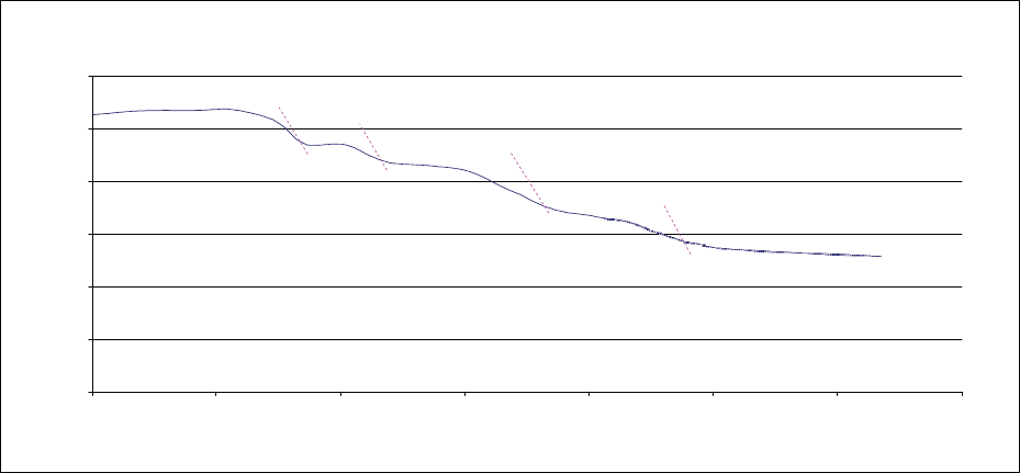
Results and Discussion: Data and Observations
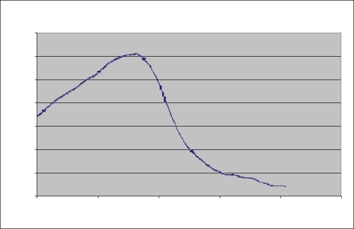
As the fault scarp profiles were examined using the updated method developed they
began to clearly fall into categories based on their overall shape. The general trend
seemed to be towards a sigmoid shape as is best typified by the profile of fault
segment 1a.

22
Figure 7: Theoretical Model of Scarp Erosion--Fault 1a Profile
The prevalence of these sigmoid shaped profiles requires an explanation. The
original state (its shape when movement stopped) of the fault scarps can be
simplified to that of a "step" in which the horizontal parts represent the pre-faulting
land surface and the angled portion represents the remnant of the fault itself as
affected by erosion. The faults associated with the rift generally have a measured dip
of -70-80° from horizontal. Assuming such an initial shape for the fault, taking into
account that this is much greater than the angle of repose for loose gravel (-30-45°),
it seems reasonable to assume that this original slope would erode in a sigmoid
fashion. That is to say that material that gets eroded out at the top of the slope
accumulates at the bottom of the slope in a debris pile or alluvial fan. This would
naturally produce a sigmoid shaped profile over time as the scarp evolves and the
original fault surface erodes. If this is the case, then the amount of material that is
missing from the top (Area 1 above) should roughly equal the amount of material in
the debris pile at the bottom of the scarp (Area 2 above), since the material that
2750
FaultPlane?
Area 1
(
eroded
)
2650
2600
2550
2500
2450
2400
Area 2
(debris)
2350
2300
0 200 400 600
800 1000 1200 1400 1600 1800
2000
23
erodes out has to go somewhere and shouldn't have the energy to make it very far.
Since a profile line is inherently 2-dimensional, this should mean that Area 1
approximately equals Area 2. This provides an important constraint on these scarp
profiles.
Other faults show features to be expected with abrupt cliffs; debris piles out beyond
the bottom of the slope. A good example of this is provided by Fault 3J. See below
corrected for Vertical Exaggeration. For a detailed discussion of vertical
exaggeration and how it is corrected see Appendix A.

Fault 3J
2750
2700
2650
2600
2550
2500
2450
2400
2350
2300
2250
0 200 400 600 800
1000
Distance(m)
1200 1400 1600 1800 2000
24
Figure
8:
Fault
3
J
Corrected
for
VE
Elevation(m)
25
Given that the small rise around the 1400 m distance mark is beyond the slope of the
scarp, it seems unlikely to be directly associated with the scarp. Given the sheer
number of faults present in this region it seems likely that this small rise is another
smaller fault within the floor of the rift. It should be noted that most of the faults
observed were the major ones that define the Rift valley, forming the Eastern and
Western Escarpments. There are many smaller faults within the valley floor with
similar or even cross-cutting (perpendicular) strikes, but with much smaller
displacement.
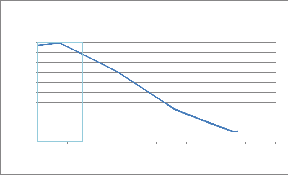
A few profiles show the odd character of being extremely crisp, appearing to be made
up of only a few straight line segments. Fault 5i seems to provide the clearest
example of this. As Excel Originally drew it:
Figure 9: Fault 5i as Drawn by Excel: Original VE
Given that this scarp has a smaller vertical drop than some of the others, a 100 meter
square was used instead of the 200 meter square used elsewhere. In any case the
vertical exaggeration (VE) isn't as big as in some of the other graphs.
Correcting for VE yields the graph below:
Fault 5i
2480
2470
2460
2450
2440
2430
2420
2410
2400
2390
2380
2370
0 50 100 150
200
Distance (m)
250 300 350 400
Elevation (m)
26
Figure 10: Fault 5i as Drawn by Excel: Corrected for VE
As can been seen, the profile appears to consist largely of straight line segments.
The slope of the lines seems to follow the general sigmoid pattern in that the steepest
one is in the middle of the scarp and the adjoining line segments are shallower. It
actually looks very much like the opposite of the theoretical model of the scarps used
in the first method. That is, breaking the scarp slope up into three slope segments;
representing the remnant scrap in the middle with the erosion surface on the left and
debris pile on the right. This scarp is likely in a fairly pristine state and perhaps
relatively young and unchanged by erosion.
Another interesting profile morphology encountered is similar to the sigmoid shape
but it has a large bump in it starting at about the mid-point of the scarp. The profile of
Fault 2n provides the best example of this:
Fault 5i
2480
2470
2460
2450
2440
2430
2420
2410
2400
2390
2380
2370
0
50 100 150
200
Distance (m)
250 300 350
400
Elevation (m)

27
Fault 2n
2740
2720
2700
2680
2660
2640
2620
2600
2580
2560
0 100 200 300 400
Dis
t
ance
(
m
)
500 600 700 800
Figure 11: Fault 2n as Drawn by Excel: Original VE
Figure 12: Fault 2n as Drawn by Excel: Corrected for VE
This one is a little harder to explain but appears very similar to scarps described in the
Northern Sector of the Kenyan Rift by Bunkley et al. Looking at the Loriu
Escarpment they argue for a sequence of events with two separate periods of faulting
and two separate emplacements of lave flows. While the second lave flow is more
specific to the area they were looking at, their explanation of that scarp seems to fit
Fault 2n
2740
2720
2700
2680
2660
2640
2620
2600
2580
2560
0100 200 300
400
Distance(m)
500 600 700
800
Elevation(m)
Elevation(m)

28
with what is seen in this profile. This implies faulting of the existing trachyte beds
followed by a quiescent period during which the scarp was eroded back and then
buried by extrusive volcanic material, followed by another period of tectonic
quiescence in which the scarp eroded back into its present shape. Perhaps it's best
to simply include their diagram of this process:
Figure 13: Buckley et al. Explanation of Development of Loriu Escarpment
29
As is explained in the accompanying text to this diagram in the book, this diagram
assumes that the geology of the area around the fault consists of a resistant cap
layer that has been worn away on the down-thrown side of the fault, underlain by a
relatively easily eroded shale. That said, A shows a young fault scarp that still bears
a reasonable resemblance to the original fault scarp after the cessation of tectonic
activity on the fault; B shows a more mature scarp in which the slope has eroded
back from the original plain of the fault; C shows the situation once a theoretical cap
of resistant rock has been removed from the up-thrown side of the fault; D shows the
terrain reduced to a pene-plain; and finally E shows the scarp re-emerging as the
erosion surface reaches a resistant underlying layer of presumably crystalline rock.
The cross-section in the upper left shows where these various erosion surfaces lie
within the cross section.
As indicated, it is not clear whether there might have been a second or even more
eruptions of material that covered the scarp after the first one, but this seems the
most likely explanation for this profile shape. Figuring out the exact eruptive history
of this scarp would require field work likely including the digging of a trench
perpendicular to the scarp to see what the underlying geology is. Given that these
are crystalline volcanic rocks, like basalt, this would likely require explosives to break
the rocks apart and thus would be both time-consuming and potentially hazardous.
Some profiles seem to hint at the possibility of re-activation in other ways. They have
a distinct bump in the middle of their slope. Fault 6a seems to provide a perfect
example of this, as seen below:
30
Figure 14: Fault 6a as Drawn by Excel: Original VE
Fault 6a
3000
2500
2000
1500
1000
500
0
0 1000 2000 3000 4000
5000
6000 7000
8000
Distance(m)
Figure 15: Fault 6a as Drawn by Excel: Corrected for VE
Fault 6a
3000
2500
2000
1500
1000
500
0
0
1000
2000 3000
4000
Distance(m)
5000 6000 7000
8000
Elevation(m)
Elevation(m)
31
Figure 16: Fault 6a Possible Interpretation
One possible explanation for the mid bump is that the slope may have been eroding
back into the classic sigmoid shape when the fault re-activated, producing the bump.
It must be remembered that visible scarps are unlikely to represent any part of the
actual fault plane and may indeed have eroded back to the point that the fault itself is
significantly displaced from the slope it created. However, in this case that
displacement would be 3 km, which seems unlikely. It's possible that this is actually
a composite scarp made of two normal faults going in opposite directions (their
strikes being 180° apart from each other). In that case this bump in the main scarp
would actually be a secondary scarp that dips in the opposite direction. The dips of
the faults in this region have been measured and are generally -70°-80° from
horizontal (Baker et al.) In the first scenario, once activity on a fault stops it is left
looking much like a step (i.e. very straight and crisp looking), the "vertical" portion of
the step being the fault itself. This is often seen around the world after a large quake
(but generally on a smaller scale); over time this crisp looking feature is eroded.
Since these faults are known to be near vertical, typically -70°-80° from horizontal, it
seems likely that some of the material from the top of the original fault scarp would be
eroded away and deposited at the bottom of the slope, leaving a debris pile. This
would leave the original trace of the fault somewhere in the middle of the slope. This
Fault 6a
3000
2500
FaultPlane?
2000
slo
p
eafte
r
firs
t
faultin
g
e
p
isode
1500
1000
500
0
0 1000 2000 3000
4000
Distance(m)
5000 6000 7000
8000
Elevation(m)
32
Fault 6e
3000
2500
2000
1500
1000
500
0
0
1000 2000 3000 4000 5000 6000 7000
Distance
(
m
)
movement of material from the top of the original scarp to its bottom would naturally
form a sigmoid shape over geologic time. If the fault were to become reactivated,
one would expect to see something very much like what's seen above. That is, a
slope somewhere between its original state and its final sigmoid shape with an
interruption to the slope at the point the fault crosses it; with the results of the erosion
of this new scarp below it.
Another general form of scarp profile observed in this research exhibited several
bumps each with sigmoid-like slopes below them. This form is best typified by the
profile of Fault 6e shown below as originally plotted in Excel:
Figure 17: Fault 6e as Drawn by Excel: Original VE
Elevation(m)
33
Fault 6e
3000
2500
2000
1500
1000
500
0
0 1000 2000 3000 4000 5000 6000 7000
Distance
(
m
)
Figure 18: Fault 6e as Drawn by Excel: Corrected for VE
As previously stated, these faults were mapped assuming that any
lineations that connected them were a continuation of the same fault and that these
faults were largely singular drops (one large slope as opposed to multiple drops &
slopes). This doesn't appear to be the case for Fault 6e. The best explanation for
this "rough and bumpy" profile, as it was originally dubbed, is that it is in fact multiple
smaller faults instead of just one large one. In this scenario each bump in the profile
would be tied to a different parallel fault.
Elevation(m)
34
Figure 19: Fault 6e Possible Interpretation
As can be seen the slope of the scarps decreases towards the bottom of the overall
slope. There are alternative interpretations for this. The first, which is displayed in
the above diagram, is that the dip of the fault planes is the same between all four
scarps, but the scarps differ in age and thus stage of erosion (i.e. the lower slope
seen in the lower faults simply reflects the fact that they are older and thus have been
eroding longer). This would also be consistent with the general dip observed for
faults within the rift. Another alternative interpretation is that the dip of the faults
changes between the faults, starting at -70°-80° near the top of slope and dropping
to -30°-40° by the bottom most fault. Still a third possibility is that this is a listric fault
system with a series of faults with decreasing dips going from left (West) to right
(East).
Limitations of Research and Future Work
Some of the limitations of this remote sensing method of observing faults should be
noted. It must be remembered that the elevation data used is based on distance
measurements taken from directly overhead. This means that a truly vertical slope
with a 90° slope would only show up as a sudden elevation change along the strike
of the slope. This can be worked around by simply assuming this to be the case
whenever such a situation is encountered.
Fault 6e
3000
Faul
t
Plane 1
Faul
t
Plane 2
2500
Faul
t
Plane 3
2000
Faul
t
Plane 4
1500
1000
500
0
01000
2000 3000 4000 5000 6000
7000
Distance
(
m
)
Eleavtion(m)
35
The other limitation is within the data itself. It must be remembered that any DEM
(Digital Elevation Model) is basically just a grid with a value for the elevation at each
point on the grid. A DEM can also be thought of as a three dimensional (3D) plot in
with each X, Y point has a corresponding Z value representing the elevation. This
creates a two dimensional surface within the 3D plot that represents the terrain in the
real world. This comes, in part, from the way in which the elevation data was
collected to begin with. The data is built up by taking distance measurements from
orbit. This is done by beaming either a radar beam or laser down at the surface.
The time it takes the spacecraft to receive the return signal from the ground is directly
proportional to the distance as in the equation below:
Equation:
Distance=half return time (since the signal travel both there and back) x the speed at
which the signal travel (for both laser and radar based systems this would be c, the
speed of light, since both are a form of electromagnetic radiation aka. Light)
Since the attitude of the spacecraft is known to a high degree of accuracy,
subtracting the distance to the ground (based on how long it takes for the signal to
return) gives the elevation of the terrain below. These measurements are generally
taken in a grid pattern with the resolution of the data being given as to how far apart
these measurement points are and how accurate each point is. In the case of the
SRTM (Shuttle Radar Topography Mission) data used, each point is accurate to
within a meter or so and the points are about 100 meters apart. In relation to this
research work, this means that a slope that is several hundred meters long will be
defined by only the couple of points at which it was measured. However, this
research only deals with the large-scale features of these scarps, so it should be well
above the resolution limits of the DEM.
It should be noted that most scarps examined in this research appear to be the result
of a sequence of events. These would include tectonic history including possible
reactivation and erosional history such as mass-wasting events. Therefore,
advanced and more detailed research is needed to categorize faults or fault
36
segments by age of development when applying the sigmoid erosion theory
hypothesized in this report.
Future work would, of course, begin with gathering "ground truthing" data, namely
going out in the field and measuring faults and slopes analyzed using this remote
sensing based method, to determine if traditional field methods such as brunton
compass support the findings of this remote sensing based method. Given the
expense involved in traveling to Kenya to measure these particular scarps, this
methodology could also be tested more locally, by using it to measure locally
accessible slopes around the Keweenaw, where a similar rifting event occurred
around a billion years ago. If the same method measures those slopes
accurately, then it's reasonable to assume that it measured the Kenyan slopes
accurately as well.
Once the "ground-truthing" is accomplished, the next logical step would be to do a
broader census of fault scarps within the rift to see if the above patterns hold more
broadly throughout the East African Rift or perhaps even beyond (to fault scarps
more generally around the world).
Conclusions
As to scarp observation, the vast majority of the fault scarps examined in this report
fell along a spectrum running from rough and shape-edged profiles indicating more
recent or active scarps to more sigmoidal profiles with each having its own subtle
eccentricities (most likely due to the anomalies of erosion such as the particular way
the bedrock breaks or an especially large landslide, or a sequence of events). This
would indicate that the scarps tend towards this state. This sigmoidal profile would
thus represent a fairly stable end-state for the erosion of these scarps.
The erosive forces on a scarp are driven by gravity; rocks and debris roll downhill and
stop rolling when the slope flattens out. This means that material eroded off the
upper portion of a scarp piles up at the bottom of the slope over time. Eventually the
slope of the debris pile, accumulating from the erosion of the upper portion of the
scarp, meets. At this point, the entire slope will be below the angle of repose and
37
stable under gravity, and thus there is no longer any force driving erosion. As the
method and observations in this report show, many of the fault profiles are variations
on the basic sigmoidal shape or are sigmoidal-shaped profiles that have been
modified through subsequent tectonic activity.
The observation method developed in this report, based on readily available remote
sensing data, can provide further evidence to support the notion that sigmoidal-
shaped profiles represent a natural endpoint of the erosional process of fault scarps.
If the sigmoidal shape is indeed an erosional end-point then one would expect these
shapes to be abundantly represented in a region such as the Southern Kenyan
portion of the East Africa Rift Valley. Over time, faults of many different ages exist
within this area. However, keeping in mind that other processes can be at work on
scarps--most notably drainage patterns, when anomalies are observed, reactivation
in some form possibly has occurred.
38
Bibliography
Dunkley, P.N., M. Smith, D.J. Allen and W.G. Darling (1993). "The geothermal activity
and geology of the northern sector of the Kenya Rift Valley", British Geological
Survey Research Report SC/93/1.
Baker, B.H. (1958). Geology of the Magadi Area. Degree Sheet 51, S.W. Quarter, pp.
1-81.
Baker, B.H. (1963). Geology of the Area south of Magadi. Degree Sheet 58, N.W.
Quarter, Report 61, pp. 1-28.
Baker, B.H., L.A.J. Williams, J.A. Miller, and F.J. Fitch. (1971). Sequence and
Geochronology of the Kenya Rift Volcanics. Elsevier Publishing Company,
Amsterdam. Tectonophysics, Vol. 11, pp. 191-215.
Baker, B.H. and J.G. Mitchell (1976). Volcanic stratography and geochronology of the
Kedong-Olorgesailie area and the evolution of the South Kenya rift valley. Geological
Society of London, Vol. 132, pp.467-484.
Reading, H.G. (1986). African Rift tectonics and sedimentation, an introduction.
Geological Society of London, Special Publications, Vol. 25, pp. 3-7.
Baker, B.H., J.G. Mitchell, and L.A.J. Williams (1988). Stratigraphy, geochronology,
and volcano-tectonic evolution of the Kedong-Naivasha-Kinangop region, Gregory
Rift Valley, Kenya. Geological Society of London, Vol. 145, pp. 107-116.
Frostick, L.E. (1997). The East African Rift basins. Elsevier Science, Vol. 3,
Amsterdam. Pp.187-209.
Atmaoui, N. and D. Hollnack (2003). Neotectonics and extension direction of the
Southern Kenya Rift, Lake Magadi area. Elsevier Publications, Tectonophysics, Vol
364. pp. 71-63.
Chorowicz, J. (2005) The East African rift system. Elsevier Publications, Journal of
African Earth Sciences, Vol. 43, pp. 379-410.
Gloaguen, R., P.R. Marpu, and I. Niermeyer (2007). Automatic extraction of faults
and fractural analysis from remote sensing data. Nonlinear Processes in Geophysics,
Vol. 14, pp. 131-138.
Ibs-von Seht, M., T. Phenefisch, and K. Klinge (2008). Earthquake swarms in
continental rifts
-
A comparison of selected cases in America, Africa and Europe.
Elsevier Publications, Tectonophysics, Vol. 452, pp. 66-77.
39
Sequar, G.W. (2009). Neotectonics of the East African Rift System : new
interpretations from conjunctive analysis of field and remotely sensed datasets in the
Lake Magadi area , Kenya Neotectonics of the East African Rift System : new
interpretations from conjunctive analysis. GeoInformation Science, February Issue,
Abstract, p.1.

40
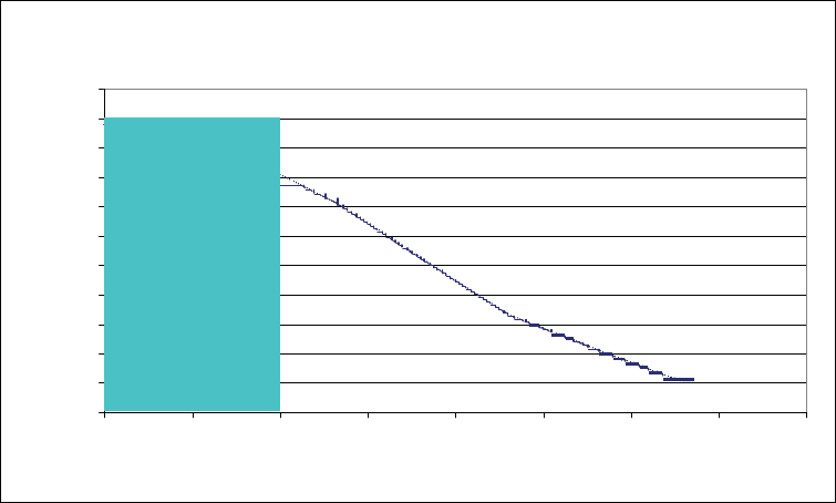
Appendix A: Vertical Exaggeration
Vertical Exaggeration (VE) is the ratio of the vertical scale to the horizontal scale
when referring to elevation. It is often useful to exaggerate elevation data because it
can make even relatively small features in the landscape stand out, making them
easier to spot and easier to analyze. When dealing with elevation plots, it is crucial to
keep VE in mind because the shape seen in the plot is not necessarily the real-world
shape. The easiest way to calculate the vertical exaggeration of a profile is to
measure the ratio of equivalent distance along the two scales with a ruler. The
distance used for this does not matter as long as the same distance is measured
along both scales. The VE of the profile is the vertical measurement over the
horizontal measurement.
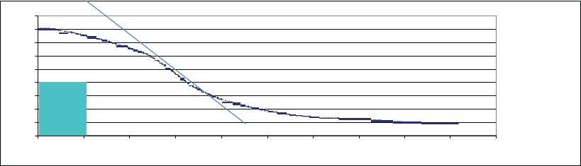
As an example, the Theoretical Model of a Fault Scarp as presented in Figure 7 in
this report is shown again below with a box for VE Explanation
Figure 20: Theoretical Model of Scarp Erosion--Fault 1a Profile: VE Example
2750
Fault Plane?
A
rea 1
(eroded)
2700
2650
2600
2550
2500
2450
2400
Area 2
(debris)
2350
2300
0
200 400
600 800 1000 1200 1400 1600 1800
2000
41
Taking this profile into account , it is apparent that the VE is substantial since the
vertical scaling is substantially less than that of the Horizontal (a given distance on
the horizontal scale represents a much large area in the real-world distance than that
same distance does on the vertical scale).
In Figure 20, a box is drawn that covers an equal scaled distance on both of the
axes. The transparency of the box is set to 75% in all graphs in this paper. The
shape of this box is dictated by the ratio of the two scales (VE). The fact that it is a
tall rectangle is indicative of the profile's substantial vertical exaggeration. If the
profile in the graph had no VE, then its shape would be that of the real world scarp.
In that case, its VE would be 1 and a box as drawn above would be a square since
the 2 scales would be equal. Given this, the graphs can be played with in Excel until
the box is square.
Since the graph starts out vertically exaggerated (stretched out of true in the vertical
direction) this can be done one of two ways: either by stretching the graph
horizontally or by compressing it vertically.
Stretching the graph horizontally, until the blue region is square, yields the following
result:
Figure 21: Fault 1a corrected for VE
2750
2700
2650
2600
2550
2500
2450
2400
2350
2300
Fault Plane?
A
rea
1
Area 2
0 200 400 600 800 1000 1200 1400 1600 1800
2000
42
As can be seen this flattens out the slope, as well as exposes the fact that the
putative fault plane line does not perfectly match up with the straight portion of the
scarp.
The VE of any graph can be calculated as the ratio of the measure distance along
each axis that represents a given scale length ("length in the real world"). If VE=1
then by definition any given length will take up the same amount of measured space
on the graph. In other words the two axis scales will be equal. The points at which
these measurements are taken along each graph are inconsequential as long as the
measure scale length is the same for both axes.
VE of graph=measured distance of vertical scale/ measured distance of horizontal
scale
Measuring the vertical axis from 2300 to 2500 meters (2500-2300=200) yields 4.1
cm, while obtaining 1.2 cm along the vertical axis measuring from 0 to 200 meters
(200-0=200).
Plugging the numbers into the above equation:
VE=4.1/1.2=3.41678
This means that all heights are exaggerated by an amount that is unique to each
graph. If VE is greater than 1 then the profile looks much steeper than it is in the real
world. Conversely, if VE is less than 1 then the graph's shape is flatter than it actually
is. All of the graphs presented in this report have a VE substantially greater than 1;
although each graph's VE differs slightly.
43
Appendix B: Excel Datasheet Containing Measurements
Fault
New
Naming
System
Segment
Strike
Steepest Slope( ° from
Horizontal)
Latitude
Longitude
1 E1 a 139.9 13.3 0.032657 N 36.394489 E
1 E1 b 163.2 6.5 0.018014 S 36.426417 E
1 E1 c 171.3 16.3 0.067172 S 36.437311 E
1 E1 d 157.6 27.9 0.164725 S 36.470681 E
1 E1 e 145 25.8 0.187347 S 36.483489 E
1 E1 f 170.6 31.3 0.211519 S 36.483506 E
1 E1 g 157.2 34.6 0.233933 S 36.505491 E
1 E1 h 148.4 37.7 0.323064 S
36.5454
E
1 E1 i 142.5 23.4 0.483508 S 36.63675 E
1 E1 J 171.4 31 0.4870324 S 36.636549 E
1 E1 k 161.6 30.7 0.5472817 S 36.6475821 E
1 E1 L 145.9 30.5 0.579314 S 36.664795 E
1 E1 m 152.8 31.2 0.62153929 S 36.691011 E
1 E1 n 175.6 48.2 0.643986 S 36.700000 E
1 E1 o 156.9 32.7 0.711344 S 36.709244 E
1 E1 p 170.9 21.5 0.747847 S 36.747847 E
2 W1 a 321.2 21 0.642741 S 36.0485448 E
2 W1 b 354.3 31.3 0.662842 S 36.0601179 E
2 W1 c 328.7 35.5 0.687056 S 36.070461 E
2 W1 d 341.6 14.3 0.707497 S 36.081942 E
2 W1 e 325.4 27.8 0.732364 S 36.09445 E
2 W1 f 349.7 19.7 0.732947 S 36.593206 E
2 W1
g 18.3 8.1 0.767353 S 36.107078 E
2 W1 h 355.4 16.8 0.794428 S 36.074869 E
2 W1 i 330.1 21.6 0.835464 S 36.110061 E
2 W1 j 5.7 14.1 0.862364 S 36.115491 E
2 W1 k 307 24.5 0.900053 S 36.125567 E
2 W1 l 5 30.3 0.920363 S 36.132467 E
2 W1 m 342.5 28 0.954169 S 36.132569 E
2 W1 n
0.7 28.3 0.995456 S 36.140628 E
2 W1 o 9.8 31.1 1.029125 S 36.137167 E
2 W1 p 11 20.9 1.058458 S 36.118705 E
3 E2 a 151 14 0.370639 S 36.376039 E
3 E2 b 165.8 16.4 0.524556 S 36.419578 E
44
3 E2 c 125.3 23.9 0.628208 S
36.468
E
3 E2 d 154.6 22.2 0.674233 S 36.504958 E
3 E2 e 156.8 20 0.750719 S 36.534478 E
3 E2 f 177 22.1 0.779508 S 36.547194 E
3 E2 g 158.9 17.1 0.317531 S 36.817467 E
3 E2 h 205.9 9.9 0.850442 S 36.554523 E
3 E2 i 163.3 30 0.77795 S 36.526239 E
3 E2 J 119.5 34.1 0.901606 S 36.572089 E
3
E2 k 173 21.9 0.934444 S 36.601244 E
4 W\2 a 350.2 21
4 W2 b 340.7 33.2 0.704581 36.110097 E
4 W\3 c 11.9 21 0.765033 36.129503 E
4 W3 d 342.3 38.5 0.799786 36.135525 E
0.2155944444
5 E3
A
169.4 14.2
S
36.611577778E
5
E3
B
183.1
16.9
0.2282138889
S
36.312558333 E
5 E3 C 152.2 13.4 0.219580556 S 36.313230556 E
5 E3 D 181.2 13.8 0.266316667 S 36.316180556 E
5 E3 E 123.7 17.2 0.29433333 S 36.318011111 E
36.3558472222
5 E3 F 177.5 19.8 0.285588889 S
E
36.3267666667
5 E3 G 128.8 25.7 0.294158333 S
E
5
E3
h
158
17.3
0.304763889 S
36.3334166667
E
0.3230722222 36.3407972222
5 E3 i 161.6 21.2
S E
0.3332416667 36.3451388889
5 E3 J 148.6 20.6
S E
5 E3 k 183.7 8.7 0.346861111 S 36.348611111 E
5
E3
L
156.7
5.8
0.3499527778
S
36.3487638889
E
5 E3 m 156.7 6.7 0.353719 S 36.3533719 E
0.3528555556
5 E3 n 116.1 10.9
S
0.35331762 E
36.3574361111
5 E3 o 178.8 9 0.358375 S
E
1.2326972222
6 W3 a 118.1 15.3 N 35.615075E
1.1116777778 35.7481694444
6 W3 b 187.1 40.7 N E
00.7598194444 35.5611722222
6 W3 c 192.4 32.8 N E
00.495972222 35.5475138889
6 W3 d 142.8 43.7 N E
6 W3 e 174.2 42.3 00.4030777778 35.5849777779
45
N
00.3399972222
E
6 W3 f 210.6 46.8 N 35.590122222 E
00.3290888889 35.5866416667
6 W3 g 185 41.1 N E
00.3116633333 35.3116333333
6 W3 h 213.6 39.2 N E
00.2928722222
6 W3 i 171 53.2 N 35.292822222 E
00.2762472222 35.2762472222
6 W3 j 213.7 52.2 N E
00.2642027778
6 W3 k 192.8 47.7 N 35.264027778E
00.258325 35.5528944444
6 W3 L 234.9 17.3 N E
00.2521333333 35.3531333333
6 W3 m 200.3 15.7 N E
7 E4 a 185.7 19.2 0.7513887 N 36.2895428 E
7 E4 b 183.2 38.8 0.6717276 N 36.2480889 E
7 E4 c 178.3 33.2 0.58019961 N 36.285513961 E
7 E4 d 193.4 35 0.55116241 N 36.284964 E
7 E4 e 233.3 32.8 0.53334679 N 36.2767425 E
7 E4 f 200 38 0.5029628 N 36.26236 E
7 E4 h 184.1 34.2 0.43658458 N 36.2590084 E
7 E4
i 177.68 44.1 0.41986382 N 36.26351055 E
46
3 E2 c 125.3 23.9 0.628208 S 36.468 E
3 E2 d 154.6 22.2 0.674233 S 36.504958 E
3 E2 e 156.8 20 0.750719 S 36.534478 E
3 E2 f 177 22.1 0.779508 S 36.547194 E
3 E2 g 158.9 17.1 0.317531 S 36.817467 E
3 E2 h 205.9 9.9 0.850442 S 36.554523 E
3 E2 i 163.3 30 0.77795 S 36.526239 E
3 E2
J 119.5 34.1 0.901606 S 36.572089 E
3 E2 k 173 21.9 0.934444 S 36.601244 E
4 W\2 a 350.2 21
4 W2 b 340.7 33.2 0.704581 36.110097 E
4 W\3 c 11.9 21 0.765033 36.129503 E
4 W3 d 342.3 38.5 0.799786 36.135525 E
0.2155944444
5 E3 A 169.4 14.2 S 36.611577778 E
5
E3
B
183.1
16.9
0.2282138889
S
36.312558333 E
5 E3 C 152.2 13.4 0.219580556 S 36.313230556 E
5 E3 D 181.2 13.8 0.266316667 S 36.316180556 E
5 E3 E 123.7 17.2 0.29433333 S 36.318011111 E
36.3558472222
5 E3 F 177.5 19.8 0.285588889 S E
5
E3
G
128.8
25.7
0.294158333 S
36.3267666667
E
5
E3
h
158
17.3
0.304763889 S
36.3334166667
E
0.3230722222 36.3407972222
5 E3 i 161.6 21.2 S E
5
E3
J
148.6
20.6
0.3332416667
S
36.3451388889
E
5 E3 k 183.7 8.7 0.346861111 S 36.348611111 E
5
E3
L
156.7
5.8
0.3499527778
S
36.3487638889
E
5 E3 m 156.7 6.7 0.353719 S 36.3533719 E
0.3528555556
5 E3 n 116.1 10.9 S 0.35331762 E
5
E3
o
178.8
9
0.358375 S
36.3574361111
E
1.2326972222
6 W3 a 118.1 15.3 N 35.615075 E
6
W3
b
187.1
40.7
1.1116777778
N
35.7481694444
E
00.7598194444 35.5611722222
6 W3 c 192.4 32.8
N
00.495972222
E
35.5475138889
6 W3 d 142.8 43.7 N E
00.4030777778 35.5849777779
6 W3 e 174.2 42.3
N
00.3399972222
E
6 W3 f 210.6 46.8 N 35.590122222 E

47
Appendix C: Estimated Error in Latitude & Longitude Measurement
Latitude and Longitude were recorded in decimal degrees and generally rounded it
off at the 6
th
decimal place.
1/100,000 of a degree of longitude is about -0.072 inches (-0.1853 cm) at the
equator (a negligible distance) given that one nautical mile equals one degree of
longitude at the equator. See math that follows.
Math:
1 Nautical Mile = 6076.12 ft = 1 minute of longitude at the equator, giving 60 NM per
degree
Therefore: 0.000001° = (60*6076.12 ft) * 0.000001 = 0.3645672 ft or 4.37486064 in
at the equator that's 0.11112 m or 11.112 cm
(1852 m *60) * 0.000001 = 0.11112m or 11.112 cm
However, the accuracy of positions was likely no more accurate than the 5
th
decimal
place or 1/100,000 of a degree; changing the co-responding numbers to 3.645672 ft
equals 43.748064 in or 111.12 cm. or -1.11 m. This accuracy measure applies the
error in Longitude only at the equator; still 33 inches is negligible on a global scale.
The error in latitude would be about the same. Since the survey area straddles the
equator, the estimates at the equator should be roughly valid across the considered
survey area. This accuracy is comparable to that of a modern GPS unit. It would be
more than sufficient to find the location of a feature in the field with a GPS unit--and
no problem to find the point within the data used or even in future datasets.
Appendix D: Fault Morphology Summary
48
Primary examples of fault morphologies in the Southern Kenya Rift are presented
below. The three faults classifications are roughly listed from suggested youngest
to most mature forms. However, most scarps examined for this report appear to
be the result of a sequence of events with separate periods of faulting and
separate emplacements of lava flows-thus difficult to categorize. Further
complication this picture are differences in the history of mass-wasting events
between fault scarps. More advanced and detailed research is needed to
categorize faults and fault segments by age, using the sigmoid endpoint theory
presented in this report.
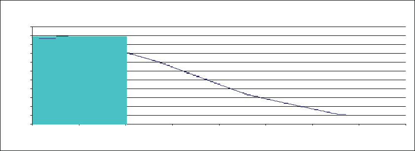
Fault Morphology 1: Youngest
-
Most "Pristine State" Fault Observed
This observed fault is likely in a fairly "pristine state" and thus appears to be a relatively
young and so far not significantly changed by erosional expected events.
Fault 5i
2480
2470
2460
2450
2440
2430
2420
2410
2400
2390
2380
2370
050
100
150
200
Distance (m)
250
300
350
400
Elevation
(m)

49
Fault Morphology 2 - Distinct Bumps - Fault Segments -Sequence of Volcanic Events
Most scarps examined as a part of this report appear to be the result of a sequence of
events with separate periods of faulting and separate emplacements of lava flow since they
are the major rift defining faults, and thus are difficult to categorize. In some cases, faulting
appears followed by a quiescent period during which the scarp was eroded and then buried
by extrusive volcanic material and then erosion again. In others, like the case above, the
escarpment appears to consist of multiple separate parallel faults, aka a fault system, as
opposed to a single larger fault. In the case above there appears to be four separate faults
along the profile line each with its own fault plane. It should be noted that each of these
fault scarps appears to be sigmoidal to the extent made possible by the fault below it.
Fault 6e
3000
Faul
t
Plane 1
Faul
t
Plane 2
2500
Faul
t
Plane 3
2000
Faul
t
Plane 4
1500
1000
500
0
0 1000 2000 3000 4000 5000 6000 7000
Distance
(
m
)
Eleavtion(m)
50
Fault Morphology 3
-
Sigmoid Angle of Repose
-
Oldest Fault
This fault appears to have eroded in a sigmoid fashion and thus appears to be older,
perhaps even at the "end-state" of erosion. Once a scarp reaches this shape it should
theoretically be stable since there's nothing left to erode by gravity from top to bottom.
Theoretically, the fault would continue to erode over geologic time, but retain its sigmoidal
shape until the whole region is eroded flat. Bearing in mind that this is a two-dimensional
slice of a three-dimensional structure, the area is roughly equivalent to volume in the
transition from 3D to 2D. The amount of material that is missing from the top (Area 1)
roughly appears to equal the amount of material in the debris pile at the bottom of the
scrap (Area 2) and thus to be at the sigmoid state. This makes sense since the material
from above has to go somewhere by gravity and the most likely place is to the bottom of
the slope where it runs out of energy to move, thus the eroded volume or area should
equal the debris pile at the bottom.
2750
FaultPlane?
Area 1
(eroded)
2700
2650
2600
2550
2500
2450
2400
Area 2
(debris)
2350
2300
0
200 400 600 800
1000 1200 1400 1600 1800
2000
